Maybe a bit carried away there, but raw data was (and is) something that needed special attention - and one of our early scale optimizations was to improve how we handled that first phase of IoT data processing.
Raw data is collected by sensors and gateways and uploaded by the gateways in a JSON format to our cloud server. While the JSON has to be well formed, there isn’t a schema or requirement of elements or structure. The JSON is also highly dependent on the hardware and firmware versions, which introduce changes to what is collected and how it is formatted.
The first priority when handling raw data is to minimize any potential for data loss, and the second priority is to respond to the gateway as soon as possible - once we can guarantee that the raw data cannot be lost even if the process fails. We want to minimize the cost of keeping the gateway waiting - in terms of cellular network costs as well as hardware battery depletion.
The next goal in raw data processing is to verify the structure and validity of the raw data and alert on issues. Finally, we want to index the raw data for future access (as may be needed) and slate it for further processing.
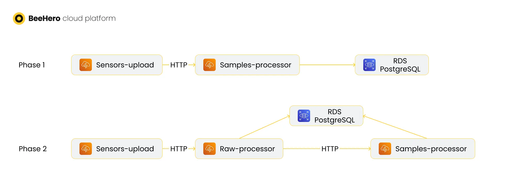
Initially the BeeHero platform was deployed as two AWS beanstalks: a .NET C# Web server - named ‘sensors_upload’ - and a monolith Python Flask Web application - the ‘api’. The gateways sent HTTP requests to the .NET sensors-upload server, which would route the various types of requests to different endpoints of the Python api server. Once the api server received a raw sample request, the code extracted the raw data from the request body and additional data from the request header, went on to validate the JSON format, handle timestamp variations, add an ‘upload_time’ attribute, serialize all the raw data to the DB ‘raw_samples’ table and set a ‘was_read’ column to True. It then launched a thread to handle the next phase of processing, and at the same time sent back a response to the sensors-upload server, which responded to the waiting gateway.
The ‘was_read’ column was used to handle processing failures - while the processing thread was triggered immediately, it would set the ‘was_read’ value to True only on successful completion. If it failed for any reason, then the row would have stayed as ‘was_read’=False, and we could re-process it later by issuing a different HTTP request that would directly call the processing code.
This process mostly worked as long as the samples’ scale was low, but when we deployed an increasing number of sensors and gateways, issues started to come up. While the initial processing of the request did not take much time, it was still limiting the Web servers’ capability to handle additional incoming requests, and we started to see HTTP timeouts on gateway requests. We also encountered cases where the request processing failed due to an unexpected request body - whether a new variation of the JSON or a malformed body - which would lead to data loss as it happened before the DB row was persisted. Finally, the DB started to become a bottleneck, as both the raw processing and the next phase processing were querying the ‘raw_samples’ tables and specifically trying to insert/update the ‘was_read’ column which locked the table rows.
To better scale the process we needed to better scale each part of it - and in order to do that we needed to separate the different components and add scalable features to each component.
We started by splitting the Python code into two independent code bases and deployed services - the raw-processor service and the samples-processor service, which retained most of the original monolith code. The new raw-processor code base was an extract of the raw data processing code from the api.
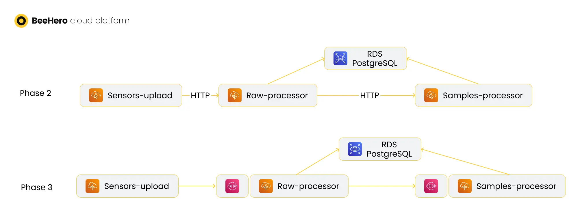
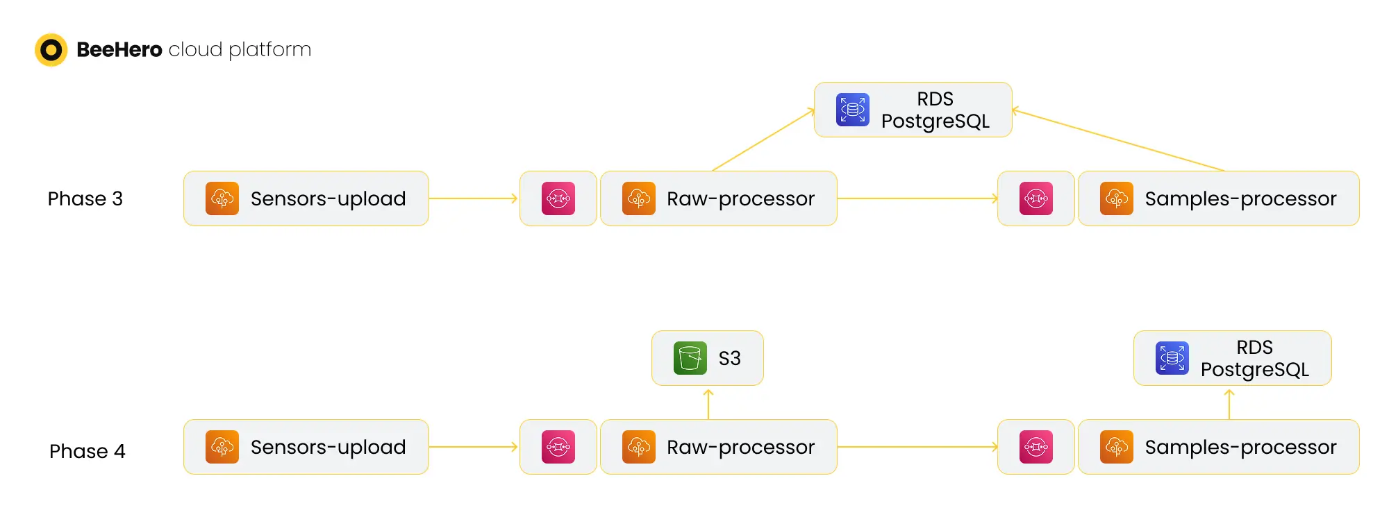
Once the deployment was completed, we changed the flow: sensors-upload will now route the HTTP request to the raw-processor Web server, which will handle the JSON validation and other tasks and then issue an HTTP request to the samples-processor for the rest of the processing (replacing the thread mechanism). The separation allowed us to scale the number of instances of each component separately, so we can scale sensors-upload and raw-processor instances to handle increased volume of requests, without the need to scale as much the heavier samples-processor server.
Then we focused on improving the hand-off between the services. Instead of relying on synchronous HTTP calls, we added AWS SQS queues before the raw-processor and samples-processor servers - AWS beanstalks can be either Web-based or queue-based, so we didn’t need to change the code to enable this transition. The transition to queues allowed us to respond to the gateway much faster - once the raw data was pushed to the raw-processor queue, we had a ‘guarantee’ that it was persisted and would be handled, so we could immediately respond to the gateway. Using AWS SQS also enabled error handling based on the deadletter queue mechanism, solving the issue of failures while processing the request body. With this change we also stopped using the Postgres table to manage what was processed - removing the reliance on the ‘was_read’ column and the resulting DB locks. Finally, the queues allowed us much greater control over scale - the raw-processor no longer had to handle all the requests as they were received, and there were no longer issues of HTTP requests being timed out.
Now that we had a reliable, scalable and fault tolerant component that handled raw samples, we were able to stop using Postgres for raw samples persistence altogether. So far Postgres was used mostly as the persistence of the raw sample until we had a processed sample, but the only queries on raw samples were for re-processing on error. Now this was taken care of via the SQS deadletter queue, and there was no longer any point in saving the raw data in Postgres - a costly storage. Instead, we moved all the raw data to S3 buckets as json files. We first transitioned the raw-processor beanstalk to save raw data to S3 instead of Postgres (the handoff to the samples processor was via the SQS message body, so it wasn’t affected), then we wrote a migration script to extract past raw samples from Postgres and saving them as S3 files, and finally we dropped the raw_samples table from Postgres. The result was moving ±2T from Postgres storage to S3 and saving hundreds of dollars per month.
A few notes on S3 as the storage medium:
* We saved each sample as a file, and organized them into partitioned folders by the raw sample’s timestamp - a hierarchy of folders (S3 path) by year, month and date
* The partitioning allowed us to efficiently index the S3 bucket using AWS Glue Catalog and query via AWS Athena, in the rare cases we needed to inspect the raw data
* S3 is scalable and reliable, so PutObject api calls very rarely fail. That being said, S3 cost is a combination of the storage used and the API calls made (i.e. PutObject API to store a file). We saved each sample separately, resulting in increased costs, which we will have to improve in our next phases (which I’ll cover in future posts)
* Another downside of saving each sample separately is the resulting file size - each file was less than 1K. This prevented us from leveraging S3 storage tiers, which are an ideal match for data which is rarely used. The reason is that AWS adds metadata for each file in order to determine the storage class, but the metadata requirement was larger than the file size, in which case AWS ‘refuses’ to transition the file to cheaper storage classes (as the increase in metadata will double the storage used)
That’s it for our raw processing scale up, at least for now - we will get back to it when we transition to Kinesis data streams later on. In the meantime, we moved on to improving the next phase in our pipeline: processed samples enrichment and storage. But that’s in our next post…